User Guide
How to Run
pyBaram provides a console script, which uses argparse module.
When you run pybaram, following help output is given:
user@Computer ~/pyBaram$ pybaram

usage: pybaram [-h] [--verbose] {import,partition,run,restart,export} ...

positional arguments:
{import,partition,run,restart,export}
                        sub-command help
    import              import --help
    partition           partition --help
    run                 run --help
    restart             run --help
    export              export --help

optional arguments:
-h, --help            show this help message and exit
--verbose, -v
pybaram import— Convert the mesh generator output to pyBaram mesh file (.pbrm). pyBaram can convert CGNS mesh (.cgns) file or Gmsh mesh file (.msh)Example:
user@Computer ~/pyBaram$ pybaram import mesh.cgns mesh.pbrm
You can also scale the mesh by appending the
-soption. For example, to scale by 0.001:user@Computer ~/pyBaram$ pybaram import mesh.cgns mesh.pbrm -s 0.001
pybaram partition— Partition a mesh file for MPI parallel computation.Example:
user@Computer ~/pyBaram$ pybaram partition <ranks> mesh.pbrm mesh_p.pbrm
You can also partition the solution files associated with a mesh file and save the results to a specified folder:
user@Computer ~/pyBaram$ pybaram partition <ranks> mesh.pbrm out.pbrs part_folder
pybaram run— Conduct flow simulation with a given mesh and configuration files (.ini).Example:
user@Computer ~/pyBaram$ pybaram run mesh.pbrm conf.ini
If you would like to conduct MPI parallel computation, please use
mpirun -n <cores>to launchpybaramscript. Note that the mesh file should be partitioned by the same number of cores.Example:
user@Computer ~/pyBaram$ mpirun -np <ranks> pybaram run mesh_p.pbrm conf.ini
pybaram restart— Restart flow simulation with a given mesh and solution files. If you would like to restart with different numerical methods, please append the configuration file.Example:
user@Computer ~/pyBaram$ pybaram restart mesh.pbrm sol-100.pbrs
pybaram export— Convert solution files to VTK unstructured grid file (.vtu) or Tecplot data file (.plt).Example:
user@Computer ~/pyBaram$ pybaram export mesh.pbrm sol-100.pbrs out.vtu
Mesh File
pyBaram can handle unstructured mixed elements; however, there are some limitations. Currently, only a single unstructured zone can be solved. It is important that volumes and faces are appropriately labeled. The volume label for a single zone should be set as fluid, and faces assigned for boundary conditions must have distinct labels.
Configuration File
The parameters for pyBaram simulation are specified in the configuration file. This file is written in the INI file format, and it is parsed using the configparser module. The following sections provide details on the sections and parameters.
Backends
The backend section configures how to run pybaram.
Currently, pybaram runs only on the CPU and there is only ‘backend-cpu’ section.
[backend-cpu]
Parameterize CPU backend with
multi-thread — for selecting the multi-threading layer. This parameter passes to
Numba.single|parallel|omp|tbbwhere
single— use only one thread for the program. This is the default value. If you are running with only MPI parallel computation, please use it. Some numerical schemes only support single thread option.parallel— use the default multi-threading layer ofNumba. Depending on the libraries,omportbbis used.omp— use OpenMP multi-threading layer.tbb— use Intel Threading building Blocks multi-threading layer.
Example:
[backend-cpu]
multi-thread = parallel
Constants
In the constants section, essential and user-defined constants are configured. Some constants can be expressed as a function of other constants. The following constants are essential, depending on the equations being solved.
gamma — ratio of the specific heats. For conventional air,
 .
All compressible equations need it.
.
All compressible equations need it.float
mu — dynamic viscosity. It should be defined when using a constant-viscosity model. This parameter is not required when viscosity is computed using Sutherland’s law.
float
Pr — Prandtl number. It should be defined for viscous simulation. For conventional air,
 .
.float
Prt — Turbulent Prandtl number. It should be defined for turbulent simulation. For conventional air,
 .
.float
Example:
[constants]
gamma = 1.4
Pr = 0.72
Prt = 0.9
Re = 6.5e6
mach = 0.729
rhof = 1.0
uf = %(mach)s
pf = 1/%(gamma)s
lref = 1.0
mu = %(mach)s/%(Re)s*%(lref)s
nutf = 4*%(mu)s/%(rhof)s
Solvers
In following sections, numerical schemes are configured.
[solver]
Type of equations and spatial discretization schemes are configured as follows.
system — type of equations.
euler|navier-stokes|rans-sa|rans-kwsstrans-<model>— Reynolds-averaged Navier-Stokes equation with turbulence model.rans-sa— one equation Spalart-Allmaras modelrans-kwsst— two-equation -SST model
order — spatial order of accuracy.
1|2gradient — method to calculate gradient. The default value is
hybrid.hybrid|least-square|weighted-least-square|green-gausslimiter — slope limiter for shock-capturing. It is configured only if the order is 2. Default value is
none.none|mlp-u1|mlp-u2u2k — tuning parameter for MLP-u2 limiter. Normally it is
 .
.float
riemann-solver — scheme to compute inviscid flux at interface.
rusanov|roe|roem|rotated-roem|hllem|ausmpw+|ausm+upviscosity — method to compute viscosity. Default value is
constant.constant|sutherland
Example:
[solver]
system = rans-kwsst
order = 2
limiter = mlp-u2
u2k = 5.0
riemann-solver = ausmpw+
viscosity = sutherland
[solver-viscosity-sutherland]
The parameters associated with Sutherland’s law can be configured as follows:
muref — Reference viscosity of the problem. See the note
float
Tref — Reference temperature of the flow (dimensional quantity).
float
CpTf — Free-stream enthalpy.
float
Ts — Sutherland temperature (dimensional quantity). Default value is 110.4 K.
float
c1 — Sutherland constant used to compute the reference viscosity (dimensional quantity). The default value corresponds to SI units at 288.15 K (
 )
)float
The quantities muref and CpTf may be specified in either dimensional or nondimensional form, depending on the flow variable configuration. The parameters Tref and Ts must be given in a consistent dimensional unit system.
If muref is provided, it is used directly as the reference viscosity in the viscosity evaluation.
If muref is not provided, it is computed from c1 and Tref using Sutherland’s law as:
In this case, CpTf must be specified in dimensional form consistent with Tref.
Example:
[solver-viscosity-sutherland]
muref = rhof*uf*lf/Re
Tref = 300
CpTf = gamma / (gamma -1)*pf/rhof
Ts = 110.4
[solver-time-integrator]
Time integration (or relaxation) schemes and related parameters are configured.
mode — steady or unsteady computation. Currently, dual-time stepping approach is not supported.
steady|unsteadycontroller — method to calculate time step size for unsteady simulation.
cfl|dtcfl — Courant - Friedrichs - Lewy Number. For unsteady simulation, it is required only for
cflcontroller. It is mandatory for steady simulations.float
dt — time step size for unsteady simulation with
dtcontrollerfloat
stepper — method to advance time step. For unsteady simulation, there are following options
eulerexplicit|tvd-rk3For steady simulation, following options can be selected.
eulerexplicit|tvd-rk3|rk5|lu-sgs|colored-lu-sgs|jacobi|blu-sgs|colored-blu-sgslu-sgs,blu-sgs— These schemes work only if disabling multi-threading layer (single).
time — initial and the last time for unsteady simulation
float, float
max-iter — the maximum iteration number for steady simulation
int
tolerance — stopping criteria for the magnitude of residual for steady simulation.
float
res-var — the residual variable to apply tolerance stopping criteria. The variable should be selected among the conservative variables. Default variable is
rho.string
coloring — the coloring strategy for colored LU-SGS scheme provided in networkx.greedy_color algorithm. Default variable is largest_first.
string
turb-cfl-factor — The factor of the
cflnumber for turbulent equations with respect to that of flow equations. It adjusts the pseudo time for turbulence equations to alleviate numerical difficulties. The default value is 1.0.string
sub-iter — The maximum iteration number for Jacobi sub-iteration process. The default value is 10.
int
sub-tol — The stopping criteria for the Jacobi sub-iteration. The default value is 0.005.
float
visflux-jacobian — The computing type of viscous Jacobian matrix for several implicit methods.
tlns|approximate|nonetlns— Based on Thin Layer Navier-Stokes equation (TLNS). Default.approximate— Based on Spectral radius. This type computes diagonal elements only.none— No viscous flux Jacobian imported. This type can cause convergence delay.Applicable methods —
jacobi,blu-sgs,colored-blu-sgs
Example for unsteady simulation:
[solver-time-integrator]
controller = cfl
stepper = tvd-rk3
time = 0, 0.25
cfl = 0.9
Example for steady simulation:
[solver-time-integrator]
mode = steady
cfl = 5.0
stepper = colored-lu-sgs
max-iter = 10000
tolerance = 1e-12
res-var = rhou
[solver-cfl-ramp]
If this section is configured, CFL number can be ramped up linearly.
Initially CFL number starts from the assigned cfl in [solver-time-integrator].
iter0— iteration until maintaining the initial CFL.int
max-iter— final iteration to finish CFL ramping.int
max-cfl— final CFLfloat
Example:
[solver-cfl-ramp]
iter0 = 500
max-iter = 2500
max-cfl = 10.0
Initial and Boundary Conditions
Following sections configure initial and boundary conditions.
The position variables (x, y, z) and
few numerical functions (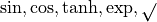 )
and constant (
)
and constant ( ) can be used.
Non-dimensionalization
pyBaram does not explicitly non-dimensionalize the governing equations. Therefore, it is recommended that users provide appropriately scaled variables for the initial and boundary conditions.
A commonly used nondimensionalization is defined as
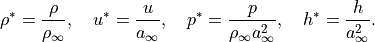
Here,  ,
,  , and
, and  denote the density, velocity, and pressure, respectively;
  denotes the speed of sound, and
  denotes the specific enthalpy.
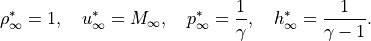
For the free-stream state, the nondimensionalized variables become
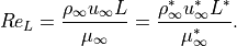
The nondimensional free-stream viscosity  is chosen to satisfy the Reynolds number
  , defined using a characteristic length
 , as
, as
This yields
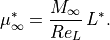
Here,  is the free-stream Mach number, and
  is the nondimensional characteristic length (e.g., the chord length used in the mesh).
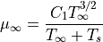
The viscosity is evaluated using Sutherland’s law in nondimensional form as
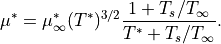
Here,  and
and  must be specified in the same dimensional unit system (e.g., Kelvin).
[soln-ics]
The initial condition is configured. All primitive variables should be configured.
Examples:
[soln-ics]
rho = rhof
u = uf*cos(aoa/180*pi)
v = uf*sin(aoa/180*pi)
p = pf
In this, examples, rhof, uf, pf and aoa are assigned at [constants] section.
[soln-bcs-name]
The boundary conditions for the label name is configured.
The label should be same as the mesh file (.pbrm).
type — type of boundary condition. To solve Euler system, following types can be used.
slip-wall|sup-out|sup-in|sub-outp|farTo solve Navier-Stokes or RANS system, following types can be used.
slip-wall|adia-wall|isotherm-wall|sup-out|sup-in|sub-outp|sub-inv|far
The details of type and required variables are summarized as follows.
slip-wall— slip wall boundary condition.adia-wall— adiabatic wall boundary condition.isotherm-wall— isothermal wall boundary condition.CpTw— wall enthalpy
sup-out— supersonic outlet boundary conditionsup-in— supersonic inlet boundary conditionall primitive variables
sub-outp— subsonic outlet boundary condition with back pressurep— back pressure
sub-inv— subsonic inlet boundary condition with velocityrho— densityu, v, w— velocity components.turbulent variables
sub-inptt— subsonic inlet boundary condition with total conditionsp0— total pressureCpT0— total enthalpydir— velocity direction components.turbulent variables
far— far boundary conditionall primitive variables
Examples:
[soln-bcs-far]
type = far
rho = rhof
u = uf*cos(aoa/180*pi)
v = uf*sin(aoa/180*pi)
p = pf

[soln-bcs-airfoil]
type = adia-wall
Plugins
Plugins in pyBaram serve as post-processing modules after iterations. If a plugin is not configured, no post-processing will occur. The following plugins can be configured:
[soln-plugin-stats]
The stats plugin writes a fundamental log file. For unsteady simulations, it includes time and time step information for each iteration. In steady simulations, it records the residuals of all conservative variables.
flushsteps— flush to file for every flushstep. Default value is 500.name— file name. If a file format is not assigned, csv format will be used by default. Default name is stats.csv
Examples:
[soln-plugin-stats]
flushstep = 300
[soln-plugin-writer]
This plugin writes the solution file.
name— file name. In the name, {n} replaces iteration number and {t} replaces time.iter-out— write solution file for every iter-out.
Examples:
[soln-plugin-writer]
name = out-{n}
iter-out = 5000
[soln-plugin-force-name]
This plugin computes aerodynamic force and moment coefficients along surface labelled name.
iter-out— compute forces for every iter-out for steady simulationint
dt-out— compute forces for every dt-out for unsteady simulationfloat
rho— reference density to compute dynamic pressurefloat
vel— reference velocity to compute dynamic pressurefloat
p— reference pressure which is subtracted from the absolute pressure. The relative pressure is integrated along the surface. The default value is zero.float
area— reference area to compute aerodynamic coefficientsfloat
length— reference length to compute aerodynamic coefficientsfloat
force-dir-name— each character (subscript) denote force direction and its direction will be configured.characters
force-dir-character — component of force direction vector of each subscript character. The dimension of this vector should same as the dimension of space.float, float, ( float )
moment-center— reference position to compute aerodynamic moment.float, float, ( float )
moment-dir-name— each character (subscript) denote moment direction and its direction will be configured.characters
moment-dir-character — component of moment direction vector of each subscript character. For two-dimensional computation, it is a scalar to indicate whether it is clockwise (-1) or counterclockwise (1). For three-dimensional computation, this vector should have the same dimension as the space.float, float, float
Examples:
[soln-plugin-force-airfoil]
iter-out = 50
rho = rhof
vel = uf
p = pf
area = 1.0
length = 1.0
force-dir-name = ld
force-dir-l = -sin(aoa/180*pi), cos(aoa/180*pi)
force-dir-d = cos(aoa/180*pi), sin(aoa/180*pi)
moment-center = 0.25, 0
moment-dir-name = z
moment-dir-z = -1
[soln-plugin-surface-name]
This plugin integrates variables along the surface labeled as name. It provides both integrated and averaged values.
iter-out— compute forces for every iter-out for steady simulationint
dt-out— compute forces for every dt-out for unsteady simulationfloat
items— items to integrate. Each item is separated by commastrings
item — expression of item. As well as reserved variables for initial and boundary conditions, nx, ny, nz, which denote the component normal vector, can be used to express item.
Examples:
[soln-plugin-surface-pout]
iter-out = 500
items = p0, mdot
p0 = p*(1+ (gamma-1)/2*(u**2 + v**2)/(gamma*p/rho))**(gamma/(gamma-1))
mdot = rho*(u*nx+v*ny)
In this example, total pressure ( ) and mass flow rate (
 ) is computed.
API
pyBaram provides an API for handling I/O and conducting simulations. Currently, only CLI (command line interface) functions are implemented. The basic usage is described as follows:
- pybaram.api.io.export_soln(mesh, soln, out)[source]
Export solution to visualization file
- Parameters:
mesh (string) – pyBaram mesh file
soln (string) – pyBaram solution file
out (string) – exported file for visualization
- pybaram.api.io.import_mesh(inmesh, outmesh, scale=1.0)[source]
Import genreated mesh to pyBaram.
- Parameters:
inmesh (string) – Original mesh from generator (CGNS, Gmsh)
outmesh (string) – Converted pyBaram mesh (.pbrm)
scale (float) – Geometric scale factor
- pybaram.api.io.partition_mesh(inmesh, outmesh, npart, solns=[])[source]
Paritioning pyBarm mesh
- Parameters:
inmesh (string) – path and name of unspliited pyBaram mesh
outmesh (string) – path and/or name of patitioned mesh
npart (int) – number of partition
solution (string) – path and name of patitioned mesh
- pybaram.api.simulation.restart(mesh, soln, cfg, be='none', comm='none')[source]
Restarted run from mesh and configuration files.
- Parameters:
mesh (pyBaram mesh) – pyBaram NativeReader object
soln (pyBaram solution) – pyBaram NativeReader object
cfg (config) – pyBaram INIFile object
be (Backend) – pyBaram backend object
comm (MPI communicator) – mpi4py comm object